TL;DR
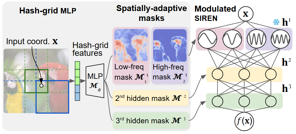
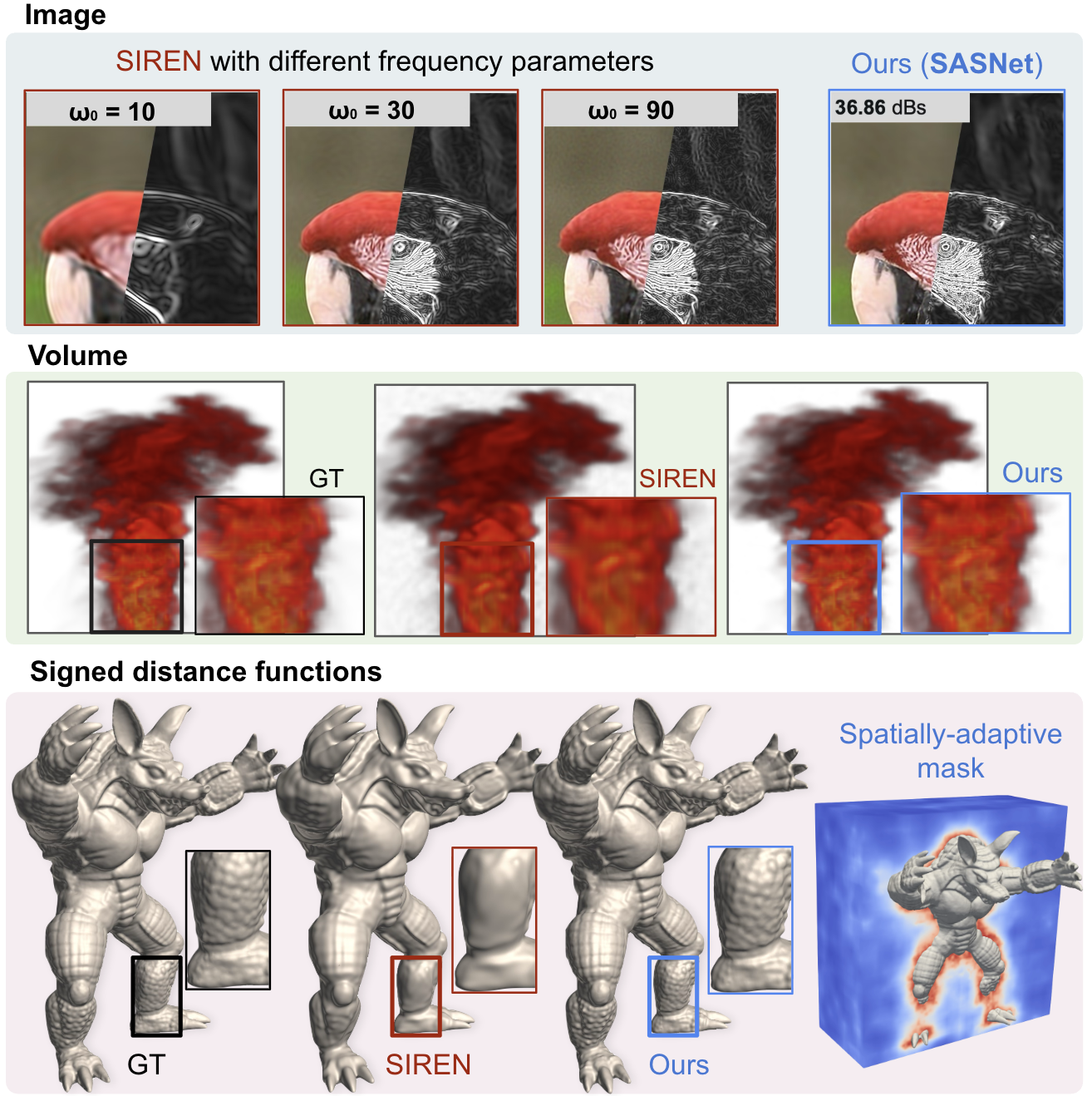
SASNet pairs a frozen frequency embedding layer with a lightweight hash-grid MLP that produces spatially-adaptive masks. The masks select, per location and per frequency band, which sinusoidal neurons express output. This suppresses high-frequency leakage in smooth regions while preserving fine detail around edges and surfaces.
A single global frequency parameter controls the entire signal. Low values produce blurry edges, while high values introduce ringing in flat regions. No per-region control is available.
Freeze the frequency embedding to fix the spectral support, and jointly learn where each frequency band is active through spatially-adaptive masks, rather than adjusting which frequencies are available.
Highest PSNR and SSIM on DIV2K and Kodak image fitting and ScalarFlow volumetric fitting, and lowest Chamfer distance with highest IoU on SDF reconstruction, with faster convergence and only modest overhead from the mask generation network.
Method
A frozen frequency embedding layer fixes the spectral support of the network, following Novello et al. (2024). In parallel, a multi-scale hash-grid MLP predicts per-layer spatial masks $\mathcal{M}^i(\mathbf{x}) \in [0,1]^{n_i}$, which modulate the sinusoidal neuron activations through an element-wise (Hadamard) product. The mask generation network and the SIREN backbone are trained jointly.
Each sinusoidal neuron in the $i$-th layer of a SIREN can be written as
$h_j^{i}(\mathbf{x}) = \sin\!\Bigg(\sum_{k=1}^{n} W_{jk}^{i}\,\underbrace{\sin(\mathbf{y}_k^{i-1})}_{h_k^{i-1}(\mathbf{x})} + b_j^{i}\Bigg)$,
where $\mathbf{y}^{i-1}$ denotes $\mathbf{h}^{i-1}(\mathbf{x})$ before activation and $W^{i}_{jk}$ controls how strongly neuron $h_k^{i-1}$ contributes to the next layer. Novello et al. (2024) show that this neuron admits the expansion
$h_j^{i}(\mathbf{x}) \;=\; \sum_{\mathbf{k}\in\mathbb{Z}^{n_i}} \alpha_{\mathbf{k}} \sin\!\Big(\langle \mathbf{k},\mathbf{y}\rangle + b_j^{i}\Big), \qquad \alpha_{\mathbf{k}} = \prod_{l} J_{k_l}(W_{jl}^{i})$,
where $J_{k_l}$ denotes the Bessel function of the first kind. The amplitudes $\alpha_{\mathbf{k}}$ depend only on the network weights, and the generated frequencies are integer linear combinations $\langle \mathbf{k}, \omega \rangle$ of the input frequencies $\omega$. Consequently, the input frequencies fully determine the spectrum of the entire network.
SASNet exploits this property by initializing $\omega$ to cover a broad spectral range, sampling most components from a low-frequency band $[-\mathcal{L}, \mathcal{L}]^{n_0}$ and the remainder from a higher band, and then freezing $\omega$ during training. Only the amplitudes $\alpha_{\mathbf{k}}$ are learned. This keeps the spectrum stable throughout optimization, in contrast to standard SIRENs whose effective frequencies drift, and accelerates convergence.
The amplitudes $\alpha_{\mathbf{k}}$ above are independent of the spatial coordinate $\mathbf{x}$, so each high-frequency component contributes globally across the domain, including in smooth regions. To localize these contributions, SASNet multiplies each neuron by a learned mask $\mathcal{M}_j^{i}(\mathbf{x}) \in [0,1]$, yielding the spatially modulated neuron
$\widetilde{h_j^{i}}(\mathbf{x}) \;=\; \mathcal{M}_j^{i}(\mathbf{x})\, h_j^{i}(\mathbf{x}) \;=\; \sum_{\mathbf{k}\in\mathbb{Z}^{n_i}} \alpha_{\mathbf{k}}\, \mathcal{M}_j^{i}(\mathbf{x})\, \sin\!\Big(\langle \mathbf{k},\mathbf{y}\rangle + b_j^{i}\Big)$.
The product $\alpha_{\mathbf{k}}\,\mathcal{M}_j^{i}(\mathbf{x})$ now plays the role of a spatially dependent amplitude: a frequency component contributes only where the corresponding mask is nonzero. Applied to the frequency embedding layer, $\mathcal{M}^1(\mathbf{x}) \odot \sin(\omega\mathbf{x} + \varphi)$ directly selects which input frequencies are visible in each region.
The masks $\mathcal{M}_\phi$ are parameterized by a small multi-scale hash-grid network (Müller et al., 2022) and trained jointly with the SIREN parameters. To control parameter count, neurons in each layer are partitioned into groups and a single mask is broadcast across all neurons within a group. In the frequency embedding layer, neurons are grouped by the magnitude of their initialized frequency; in hidden layers, neurons are partitioned evenly.
Results · 2D images
| Method | PSNR ↑ | SSIM ↑ | PSNRedge ↑ | Noisiness ↓ |
|---|---|---|---|---|
| SIREN | 34.64 | 0.959 | 31.37 | 2.525 |
| FFN | 31.92 | 0.910 | 30.20 | 9.873 |
| SAPE | 32.57 | 0.932 | 30.31 | 3.128 |
| WIRE | 28.76 | 0.831 | 25.73 | 10.324 |
| FINER | 37.52 | 0.967 | 34.02 | 4.617 |
| GaussianImage | 37.38 | 0.973 | 33.25 | – |
| NeuRBF | 36.33 | 0.959 | 33.92 | 6.975 |
| SASNet (Ours) | 39.82 | 0.979 | 36.81 | 2.105 |
Best / runner-up. SASNet wins on all four metrics, with the largest gap on noisiness: direct evidence that the masks suppress frequency leakage.
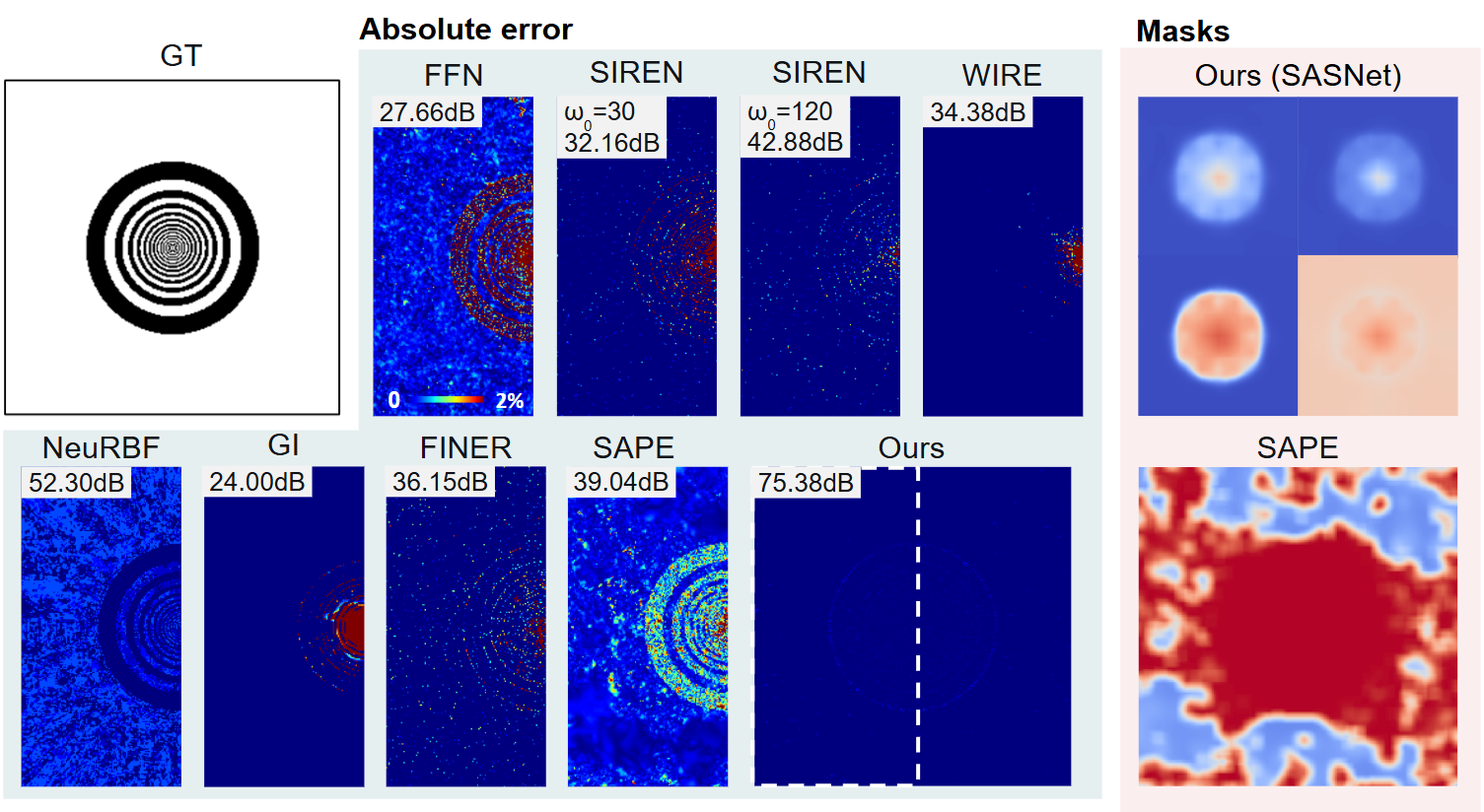
Error maps and learned masks on a toy image. Most baselines exhibit ringing or fail to capture the central high-frequency structure. SASNet learns well-localized, multi-frequency masks that activate only where they are needed, in stark contrast to SAPE's spatially inconsistent masks.
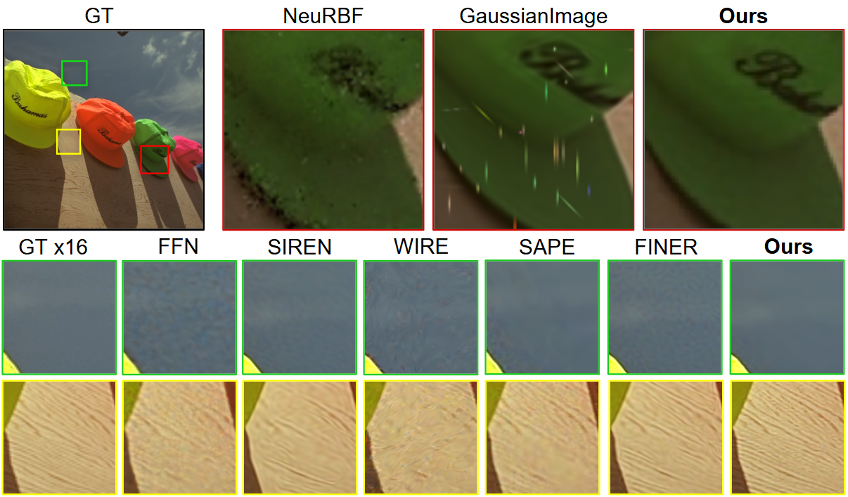
Pixel shift and ×16 super-resolution. SASNet is the only method that simultaneously preserves sharp texture (yellow boxes) and stays clean in smooth regions (green boxes).
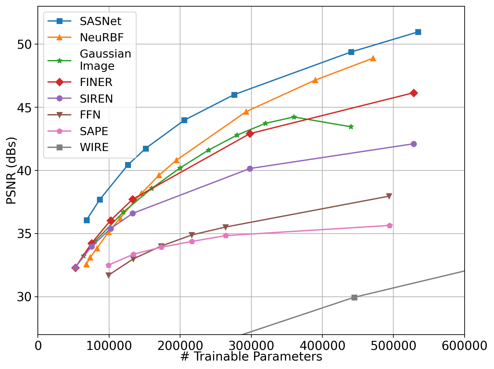
Scalability on Kodak. SASNet shows good scaling behavior, leading across the practical parameter range.
Results · 3D volumes
| Method | PSNR ↑ | SSIM ↑ |
|---|---|---|
| PEMLP | 40.42 | 0.9434 |
| Gauss | 47.11 | 0.9920 |
| SIREN | 47.67 | 0.9948 |
| FINER | 49.77 | 0.9959 |
| WIRE | 53.06 | 0.9963 |
| SASNet (Ours) | 55.92 | 0.9973 |
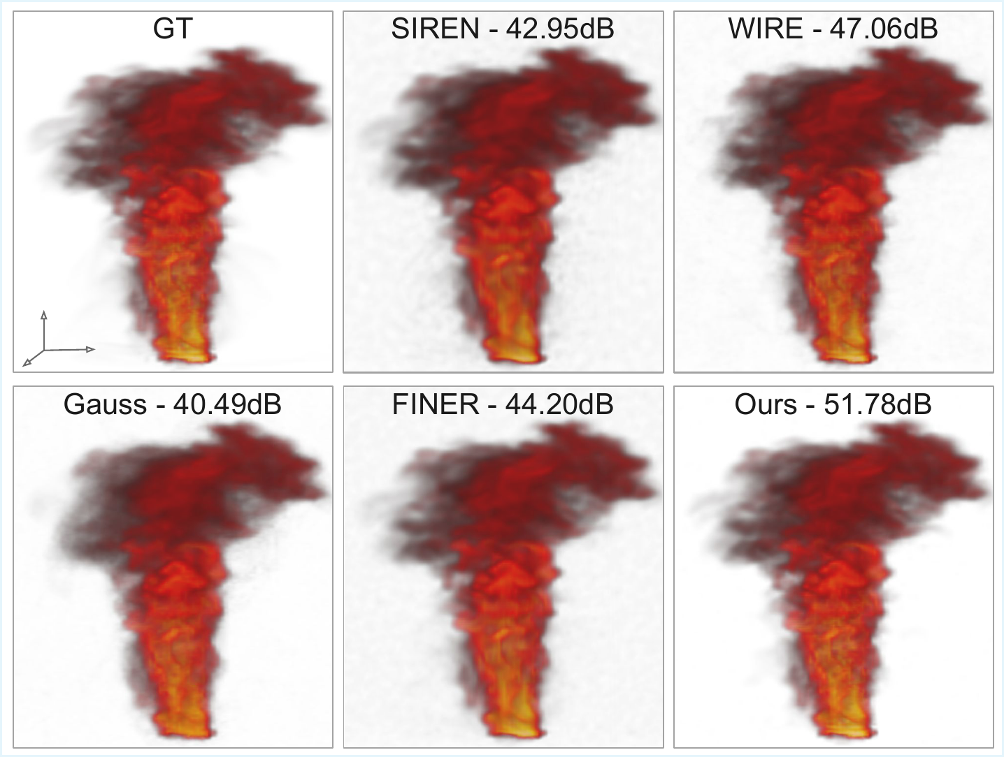
SASNet recovers thin filaments and turbulent detail while keeping a clean empty background, whereas global methods (SIREN, FINER) leak high-frequency noise into empty regions and local methods (WIRE) introduce artifacts in smooth areas.
Results · Signed distance fields
Drag to rotate, scroll to zoom. Each mesh is the zero-level set of the SDF learned by the corresponding method, extracted with Marching Cubes and decimated for web display. The two viewers are independent, so you can pick any pair of methods to compare directly on the same shape.
SIREN · Chamfer: 2.871 × 10⁻⁶ · IoU: 0.9694
SASNet (Ours) · Chamfer: 1.964 × 10⁻⁶ · IoU: 0.9809
Meshes decimated to ~120K faces from the original ~600K-face reconstructions for web delivery.
| Metric | Method | Armadillo | Dragon | Lucy | Thai Statue | Avg. |
|---|---|---|---|---|---|---|
| Chamfer ↓ (×10⁻⁶) | PEMLP | 3.465 | 2.039 | 2.387 | 4.460 | 3.088 |
| Gauss | 7.283 | 13.04 | 11.78 | 11.62 | 10.93 | |
| SIREN | 3.599 | 2.871 | 2.405 | 4.381 | 3.314 | |
| WIRE | 3.274 | 2.172 | 2.419 | 3.296 | 2.790 | |
| FINER | 4.040 | 2.477 | 2.536 | 4.201 | 3.313 | |
| SASNet | 3.368 | 1.964 | 1.927 | 3.090 | 2.587 | |
| IoU ↑ | PEMLP | 0.9878 | 0.9803 | 0.9677 | 0.9561 | 0.9730 |
| Gauss | 0.9806 | 0.9561 | 0.9581 | 0.9418 | 0.9592 | |
| SIREN | 0.9872 | 0.9694 | 0.9716 | 0.9561 | 0.9711 | |
| WIRE | 0.9910 | 0.9747 | 0.9693 | 0.9635 | 0.9746 | |
| FINER | 0.9837 | 0.9728 | 0.9671 | 0.9518 | 0.9689 | |
| SASNet | 0.9891 | 0.9809 | 0.9813 | 0.9654 | 0.9792 |
SASNet leads on the Chamfer / IoU average across four canonical shapes.
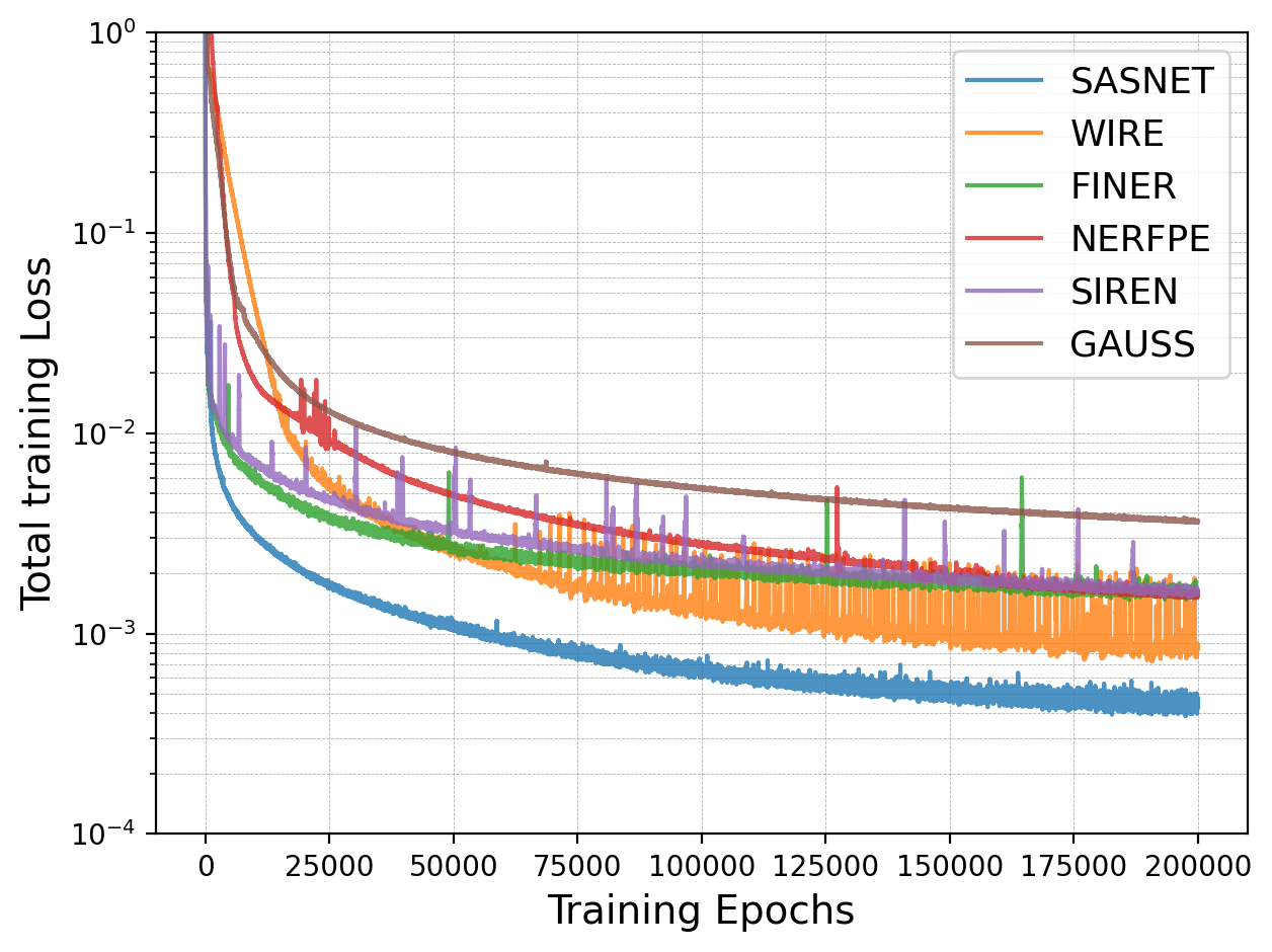
Convergence: SASNet reaches the final loss of the strongest baseline within the first ~35K iterations, then keeps improving.
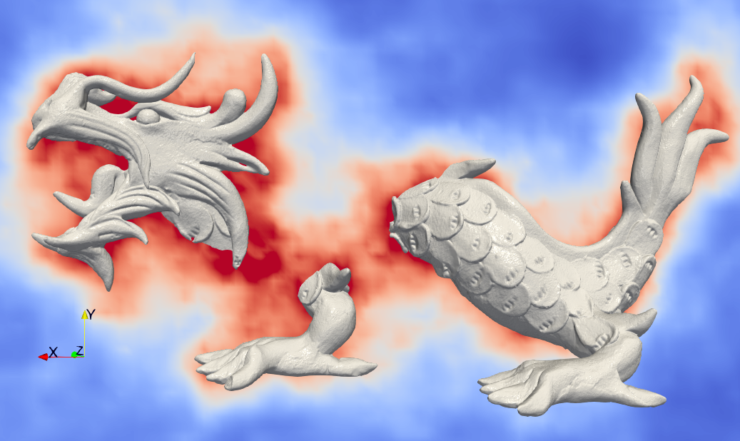
What the masks learn: a sliced view of the highest-frequency mask shows activation concentrating tightly around the zero-level set, exactly where high-frequency detail is needed.
@inproceedings{feng2026sasnet,
title = {SASNet: Spatially-Adaptive Sinusoidal Neural Networks},
author = {Feng, Haoan and Aldana, Diana and Novello, Tiago and De Floriani, Leila},
booktitle = {Proceedings of the IEEE/CVF Conference on Computer Vision and Pattern Recognition (CVPR)},
year = {2026}
}